An Introduction to Stiff ODEs with Matlab

7 minute read

Notice: The python version of this post can be found here.

Info: The solver interfaces provided by Matlab and SciPy are not exactly the same (SciPy uses rtol*abs(y)+atol while Matlab uses max(rtol*abs(y),atol)), so we will use different solvers and tolerances. . If you are interested, please refered to the SciPy document and the Matlab document.

It’s well-known that stiff ODEs are hard to solve. Many books are written on this topic, and Matlab even provides solvers specialized for stiff ODEs. It is easy to find resources, including the wikipedia entry, with technical and detailed explanations. For example, one of the common descriptions for stiff ODEs may read:

An ODE is stiff if absolute stability requirement is much more restrictive than accuracy requirement, and we need to be careful when we choose our ODE solver.

However, it’s fairly abstract and hard to understand for people new to scientific computing. In this post, I hope to make the concept of stiffness in ODEs easier to understand by showing a few Matlab examples. Let’s start with a simple (non-stiff) example, and compare it with some stiff examples later on.

Example 1

Let’s consider a non-stiff ODE

$\textrm{y'}=\textrm{Ay}$

where $A=\lambda$

In the first case we have $\lambda \;=-0\ldotp 1$ . The solution is

$y\left(t\right)=e^{-0\ldotp 1t} y\left(0\right)$ ,

meaning we have a exponential decaying function. We can look at the solution from ode45:

lambda = -1e-1;
A = lambda;
F = @(t,u) A*u;

% set the initial value to one
u0 = ones(size(A,1),1);
% time interval
t = [0 10];

% set up the axes limite
xL = [0 max(t)];
yL = [-0.1 max(u0)];

ode45

[T, Y] = ode45(F, t, u0);
plot(T, real(Y),'-o');
axis([xL, yL])
title('ODE45')

xlabel('t')
ylabel('y')

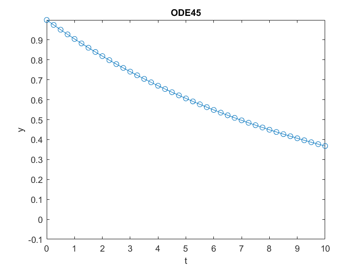
As we can see, as expected ode45 gives us a decaying function. In this interval, ode45 used

length(T)

ans = 
    41

steps to achieve the default error tolerance.

Example 2

Let’s consider the same equation

$\textrm{y'}=\textrm{Ay}$

but now $A=\left\lbrack \begin{array}{cc} \lambda_1 & \\ & \lambda_2 \end{array}\right\rbrack$

In the first case we have $\lambda_1 =-0\ldotp 1,\;\lambda_2 ={10}^3 \lambda_1$ . This means we have two decoupled equations. The solution is

$y\left(t\right)=\left\lbrack \begin{array}{c} y_1 \left(t\right)\\ y_2 \left(t\right) \end{array}\right\rbrack =\left\lbrack \begin{array}{c} e^{-0\ldotp 1t} y_1 \left(0\right)\\ e^{-100t} y_2 \left(0\right) \end{array}\right\rbrack$ ,

meaning we have two exponential decaying functions. We can use ode45 to solve it in the same fashion:

lambda1 = -1e-1;
lambda2 = 1e3*lambda1;
A = diag([lambda1, lambda2]);
F = @(t,u) A*u;

% initial value
u0 = ones(size(A,1),1);
% time interval
t = [0 10];

% set up the axes limit
xL = [0 max(t)];
yL = [-0.1 max(u0)];

ode45

[T, Y] = ode45(F, t, u0);

plot(T, Y,'-o');
axis([xL, yL])
title('ODE45')

legend({'y_1','y_2'})

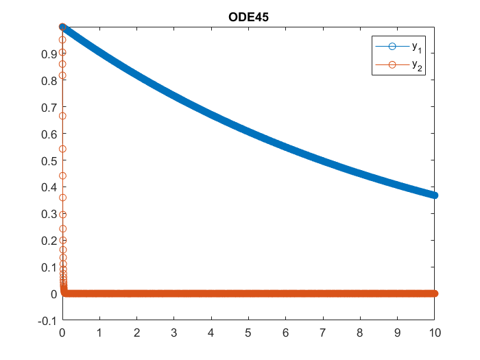
This time we get 2 decaying functions, and $y_2$ decays much faster then $y_1$ . In this same interval, ode45 used

length(T)

ans = 
        1257

steps to achieve the default error tolerance. In this example, $y_1$ is exactly the same as the solution in Example 1, but it take much longer to calculate. One may think the step size of ode45 is limited by the accuracy requirement due to the addition of $y_2$ . However, this is clearly not the case since $y_2$ is almost identically $0$ on the entire interval. What is happening here is that, the step size of ode45 is limited by the stability requirement of $y_2$ , and we call the ODE in Example 2 stiff.

Matlab provides specialized ODE solvers for stiff ODEs. Let’s look at ode15s

ode15s

[T, Y] = ode15s(F, t, u0);

plot(T, Y,'-o');
axis([xL, yL])
title('ODE15s')

legend({'y_1','y_2'})

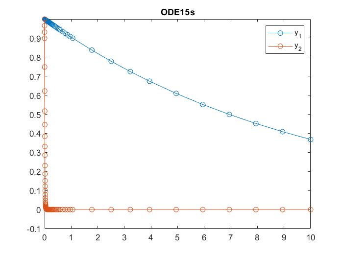
This time ode15s takes

length(T)

ans = 
    81

steps. Apparently, ode15s is significantly more efficient than ode45 for this example. From the figure above, we can also see that ode15s stratigically used shorter step size when $y_2$ is decaying fast, and larger step size when $y_2$ flattens out.

At this point you may think that if you don’t know whether an ODE is stiff or not, it is always better to use ode15s. However, this is not the case, as we will show in the next example.

Oscillatory ODE

Example 3

Let’s look at an oscillatory ODE

$\textrm{y'}=Ly$

and $L=\left\lbrack \begin{array}{cc} & \lambda \;\\ -\lambda \; & \end{array}\right\rbrack ,\;\lambda =-0\ldotp 1$

The eigenpairs of $L$ are

$\left(\pm \lambda i\;,\left\lbrack \begin{array}{c} 1\\ \pm i \end{array}\right\rbrack \right)$

The solution is oscillatory because the eigenvalues are imaginary. Let’s look at the solution from ode45

lambda = 1e-1;
L = [zeros(size(lambda)) lambda; -lambda zeros(size(lambda))];
F = @(t,u) L*u;

% initial value
u0 = ones(size(L,1),1);
% time interval
t = [0 50];

% set up the axes limite
xL = [0 max(t)];
yL = [-2*max(u0) 2*max(u0)];

ode45

[T, Y] = ode45(F, t, u0);

plot(T, Y,'-o');
axis([xL, yL])
title('ODE45 oscillatory')

legend({'y_1','y_2'})

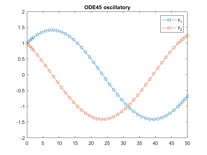
length(T)

ans = 
    45

As expected, we see two (slow) oscillatory functions.

Example 4

Now let’s look at a stiff oscillatory ODE

$\textrm{y'}=Ly$

and $L=\left\lbrack \begin{array}{cc} & A\\ -A & \end{array}\right\rbrack ,\;A=\left\lbrack \begin{array}{cc} \lambda_1 & \\ & \lambda_2 \end{array}\right\rbrack$

The eigenpairs of $L$ are

$\left(\pm \lambda_1 i,\left\lbrack \begin{array}{c} 1\\ 0\\ \pm \;i\\ 0 \end{array}\right\rbrack \right)$ , and $\left(\pm \lambda_2 i,\left\lbrack \begin{array}{c} 0\\ 1\\ 0\\ \pm i \end{array}\right\rbrack \right)$

Similar to before, we set $\lambda_1 =0\ldotp 1,\lambda_2 =100\lambda_1$ . Now we have both fast and slow oscillatory functions in our solution.

lambda1 = 1e-1;
lambda2 = 1e2*lambda1;
A = diag([lambda1, lambda2]);
L = [zeros(size(A)) A; -A zeros(size(A))];
F = @(t,u) L*u;

% initial value
u0 = ones(size(L,1),1);
% time interval
t = [0 50];

% set up the axes limite
xL = [0 max(t)];
yL = [-2*max(u0) 2*max(u0)];

ode45

[T, Y] = ode45(F, t, u0);

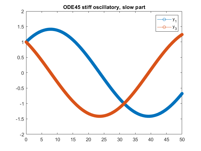
plot(T, Y(:,[1 3]),'-o');
axis([xL, yL])
title('ODE45 stiff oscillatory, slow part')

legend({'y_1','y_3'})

h = plot(T, Y(:,[2 4]),'-o');
axis([xL, yL])
title('ODE45 stiff oscillatory, fast part')

legend({'y_2','y_4'})

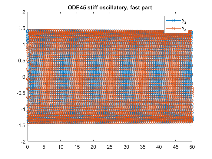
In the plots we can see both slow and highly oscillatory parts. Again, similar to the decaying case, now ode45 is taking shorter step sizes because of the the fast oscillating part, even though and could have taken much shorter time steps like the example above. In this case,

length(T)

ans = 
        2553

ode15s

[T, Y] = ode15s(F, t, u0);

plot(T, Y(:,[1 3]),'-o');
axis([xL, yL])
title('ODE15s stiff oscillatory, slow part')

legend({'y_1','y_3'})

plot(T, Y(:,[2 4]),'-o');
axis([xL, yL])
title('ODE15s stiff oscillatory, fast part')

legend({'y_2','y_4'})

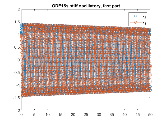
length(T)

ans = 
        1711

This time there are two issues with ode15s. First, the saving is not huge comparing to the non-oscillatory example. Second, it adds visible artificial damping to the solution, and the accuracy suffers. It it more apparent in plot all the solutions.

plot(T, Y,'-o');
axis([xL, yL])
title('ODE15s stiff oscillatory, artificial damping')

legend({'y_1','y_2','y_3','y_4'})

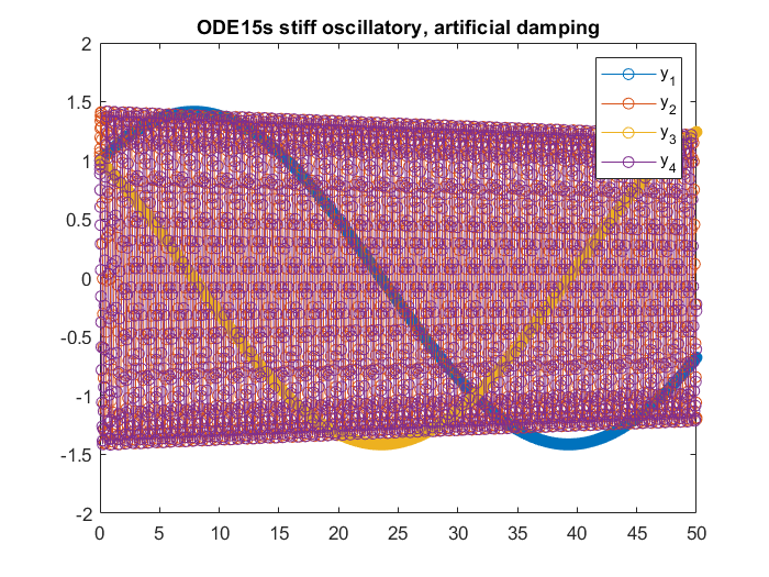
Actually, the same damping phenomenon appears with ode45, but it’s not significant.

ode23t

In the oscillatory case, we can use ode23t if the artificial damping demonstrated above is undesirable. However, it can take very short time steps and become very expensive in order to control the accuracy for the highly oscillatory components.

[T, Y] = ode23t(F, t, u0);

h = plot(T, Y(:,[1,3]),'-o');
axis([xL, yL])
title('ODE23t stiff oscillatory, slow part')

legend({'y_1','y_3'})

plot(T, Y(:,[2 4]),'-o');
axis([xL, yL])
title('ODE23t stiff oscillatory, fast part')

legend({'y_2','y_4'})

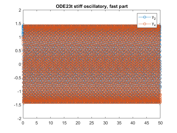
length(T)

ans = 
        4581

Notice highly oscillatory and stiff ODEs are generally hard to solve. Both ode15s and ode45 will add artificial damping to the solution. ode23t is non-dissipative, but short step size must be used, making it much more costly.

This blog post is published at https://edwinchenyj.github.io. The pdf version and the source code are available at https://github.com/edwinchenyj/scientific-computing-notes.

Share on

Twitter Facebook LinkedIn

An Introduction to Stiff ODEs with Matlab

Example 1

ode45

Example 2

ode45

ode15s

Oscillatory ODE

Example 3

ode45

Example 4

ode45

ode15s

ode23t

Share on

Leave a comment

You may also enjoy

Simple speed up for the LDLT solver

Deploy static threejs site on Github Pages

An Introduction to Compiling C++ projects, Part 2

An Introduction to Compiling C++ projects, Part 1